AFMIS

Advanced Fisheries Management Information System

REAL-TIME FORECAST

DEMONSTRATION OF CONCEPT PLAN

Georges Bank: 15 March - 15 April 2000

Brian J. Rothschild

Lead Principal Investigator - CMAST

Allan R. Robinson

Principal Investigator - Harvard, Demonstration Chief Scientist

Merlin Miller

Principal Investigator - Physical Sciences, Inc.

 

Hyun-Sook Kim

Editor - CMAST

Wayne G. Leslie

Editor - Harvard

 

NASA --- ONR

 

---

Table of contents

Preface

1. Executive Summary
2. Goals and Objectives
3. Schedule and Products
4. Protocols and Logistics
5. Observation System Simulation Experiments (OSSE): Design and Execution
6. Resources

Appendix 1 - List of Acronyms

Appendix 2 - Hypotheses, research issues, concepts and processes

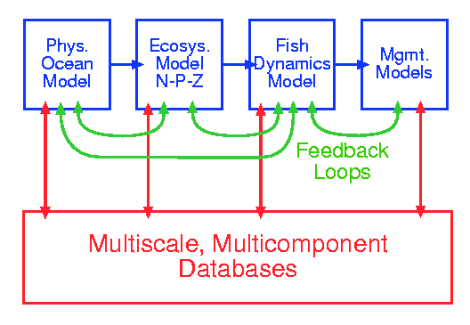
The Advanced Fisheries Management Information System (AFMIS) is intended to apply state-of-the-art multidisciplinary and computational capabilities to high-frequency operational fisheries management. The system development concept is aimed toward: 1) utilizing information on the "state" of ocean physics, biology, and chemistry; the assessment of spatially-resolved fish-stock population dynamics and the temporal-spatial deployment of fishing effort to be used in the operational management of fish stocks; and, 2) forecasting and understanding physical and biological conditions leading to recruitment variability. Systems components are being developed in the context of using the Harvard Ocean Prediction System to support or otherwise interact with the: 1) synthesis and analysis of very large data sets; 2) building of a multidisciplinary multiscale model (coupled ocean physics/N-P-Z/fish dynamics/management models) appropriate for the northwest Atlantic shelf, particularly Massachusetts Bay and Georges Bank; 3) the application and development of data assimilation techniques; and, 4) with an emphasis on the incorporation of remotely sensed data into the data stream.

This nowcasting and forecasting exercise is intended to demonstrate important aspects of the AFMIS concept by producing real time coupled forecasts of physical fields, biological and chemical fields, and fish abundance fields. Forecasts in three spatial dimensions of ten days duration will be produced once a week for a month. It is intended to verify the physics, to validate the biology and chemistry but only to demonstrate the concept of forecasting the fish fields, since the fish dynamical models are at a very early stage of development. In addition, it is intended to demonstrate the integrated system concept and to consider the implication of coupling a management model. A ten day duration forecasts was chosen to shorten the management decision times and to lengthen fishing boat planning times. Since weather forecasts are not at all reliable after five days, the second half of the physical forecasts will reflect only internal sea dynamics.

1. Executive Summary

The Advanced Fisheries Management Information System (AFMIS) will apply state-of-the-art multidisciplinary and computational capabilities to fishing and fisheries management. AFMIS is unique for several reasons. Coupled physics and biochemical dynamics has been previously accomplished. The addition of fish dynamics provides a new and potentially very valuable capability. AFMIS is designed to model a large region consisting of most of the North West Atlantic. Several smaller domains, including the Gulf of Maine and Georges Bank are nested within this larger domain. This provides a capability to zoom into these domains with higher resolution while maintaining the essential physics which are coupled to the larger domain. AFMIS will be maintained by the assimilation of a variety of real time data. Specifically this includes sea surface temperature (SST), color (SSC), and height (SSH) obtained from several space-based remote sensors (AVHRR, SeaWiFS and Topex/Poseidon). The assimilation of these data will allow nowcasting and forecasting over significant periods of time.

This document provides a detailed plan for a first demonstration of a complete AFMIS. The goals are 1) to demonstrate real-time nowcasting and forecasting of coupled physical, biochemical and fish distribution fields on Georges Bank for a period on the order of 1 to 2 weeks and 2) utilize the data obtained to produce information relevant to fisheries management. These goals are based on several hypotheses, including the assumption that a dedicated ocean prediction system (AFMIS) which properly incorporates the interaction processes and feedback between the three dynamics can nowcast and forecast state variables of interest and that fish abundance distributions vary over 1 to 2 week time scales in ways that are important for fisheries management and fishing. The demonstration of concept (DOC) has been structured to directly address these hypotheses by providing results in near real time to a variety of users.

This DOC is scheduled for the time period from about 15 March 2000 to 15 April 2000. During this 1-month period, forecasts will be issued on a weekly basis. Each of these forecasts will provide prediction of the various fields for the subsequent ten days.

The specific products which will be issued include the following:

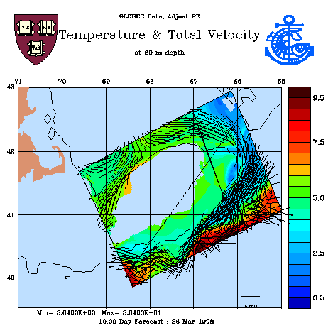
· Synoptic maps at three levels (surface, mid-level, bottom) at 1200 local time for: temperature, salinity, current speed (sub-tidal), velocity vectors (sub-tidal), Herring abundance, Cod abundance, chlorophyll, nutrients, zooplankton and surface-bottom velocity difference (sub-tidal).

· One map containing plots of total (tidal and sub-tidal) velocity

· Daily mean surface plots of total (tidal and sub-tidal) velocity

· Daily mean surface circulation, with overlying temperature, at 1200 local time

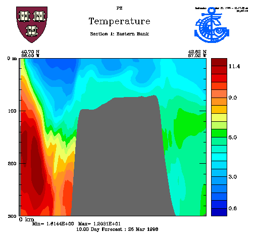
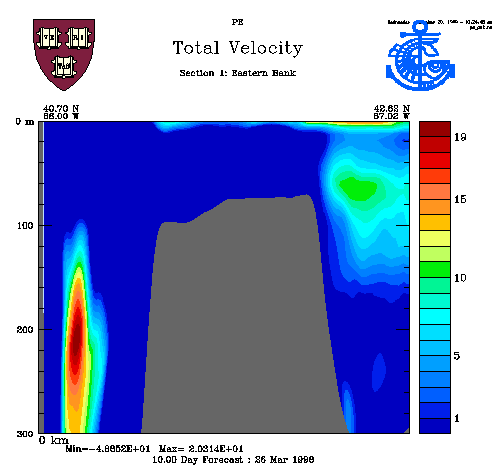
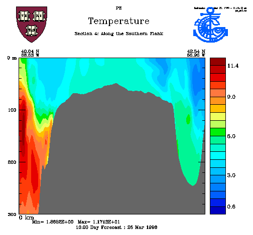
· Two vertical sections (along Georges Bank and across the bank) of temperature and velocity

· Daily mean circulation (sub-tidal) at two levels (surface and bottom) for the Gulf of Maine domain.

Other products may also be issued if warranted and of interest to the user community.

A number of technical tasks must be accomplished prior to the DOC. The coupled physical and biochemical models are available but need to be tuned to the March/April conditions on Georges Bank. Additional work on the fish dynamics model is required prior to its full integration. Some details of the nesting procedures also require additional development.

Data required to support AFMIS are obtained from a number of sources, generally via the Internet. Protocols for the collection of satellite data (SST, SSC, and SSH) and other data have been specified and individually tested. Quality control and preparation procedures have been specified.

All models will be fully developed and integrated by 1 January 2000. Starting in October, a number of Observation System Simulation Experiments (OSSE) will be accomplished to test several critical aspects of AFMIS. These will include:

· New real-time data acquisition

· Data quality control/preparation and analysis of gridded fields

· Calibration of physical and numerical parameters

· Product generation.

Given success with these OSSEs, pre-operational forecasting will be started about 15 February. This will provide experience with real-time operation and allow procedures and operations to be optimized prior to the actual DOC.

Upon completion of the DOC, a critical evaluation of the results will be undertaken. The objectives of this activity will be to assess the operational aspects of AFMIS, determine the utility of the products and to identify modifications to models and/or procedures which will optimize performance and enhance the utility of AFMIS.

2. Goals and Objectives

• To demonstrate in real-time the nowcasting and forecasting of coupled physical, biogeochemical, and fish distribution fields (as functions of x, y, z and t) in an area encompassing Georges Bank for fisheries management on the order of 1-2 weeks.

• To utilize the data obtained from the coupled physical, biogeochemical, and fish distribution fields to produce fisheries management information.

• Test and improve dynamical hypotheses (physical, biology, fish)

1. There are important interactive processes between the physics, biology and fish dynamics and feedbacks.
2. The variations in fish abundance over 1-2 week time scales are important for fisheries management and fishing.
3. A fisheries dedicated ocean prediction system can nowcast and forecast the state variables of interest.

• Explore implications of knowledge of fish fields

• Tune, evaluate and evolve the system concept, system components and integration

• Facilitate communication and feedback between managers and forecasters

• Verifiable physics

• Valid biology

• Demonstrate fish (Mark (-1)) model concept and forecast

• Use above to consider client input/output

• Model input/output commercial fishing regulations/recommendations

3. Schedule and Products

The AFMIS Real-Time Demonstration of Concept (RTDOC) is scheduled for the nominal time period 15 March - 15 April 2000. This one-month long time period will have four (4) forecast issue dates. Ten day long forecasts will be issued on a weekly basis. The first "internal trial" forecast (with a nowcast of 15 March and a first day forecast of 16 March) will be available for evaluation late in the day on 15 March. Actual forecast issue dates will be 22 and 29 March and 6 and 13 April.

The AFMIS operational system should be in place by 1 January 2000. This provides a six-week time window in which to identify and repair problems which may occur in the model system. This schedule also allows for time to modify operational protocols based on the synoptic oceanographic conditions, logistical considerations and OSSE results.

CMAST will be the site from which AFMIS operational products are distributed. The methods by which the products will be released are: a web site based distribution, email summaries to identified users and fax. Overnight delivery of hardcopy will be sent to critical persons, while standard US mail delivery (2-3 days) will be utilized for other recipients. The standard operational products for the Georges Bank region will be issued for a ten-day period with products on a daily basis during that period. The products will include:

• Synoptic maps at three levels (Surface, Mid-level, Bottom) at 1200 local time for: temperature, salinity, current speed (sub-tidal), velocity vectors (sub-tidal), Herring abundance, Cod abundance, chlorophyll, nutrients, zooplankton and surface-bottom velocity difference (sub-tidal)
• One map containing plots of total (tidal and sub-tidal) velocity (actual product is being designed)
• Daily mean surface circulation (sub-tidal), with overlying temperature, at 1200 local time
• Two vertical sections (along Georges Bank and across the bank) of temperature and velocity
• Daily mean circulation (sub-tidal) at two levels (Surface and Bottom) for the Gulf of Maine domain region
• Additional fisheries management information (to be determined through interactions with the external board of advisors)

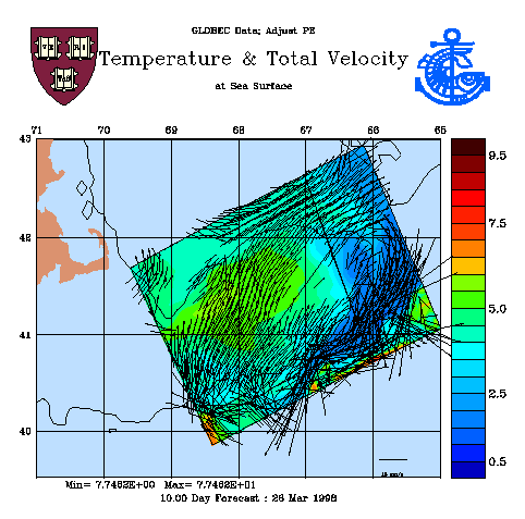
Some example products for a Georges Bank forecast can be found below.

4. Protocols and Logistics

The central dynamical models for the AFMIS RTDOC are contained with the Harvard Ocean Prediction System (HOPS). HOPS (see Figure 1a) is a flexible, portable and generic system for inter-disciplinary nowcasting, forecasting and simulations. HOPS can rapidly be deployed to any region of the world ocean, including the coastal and deep oceans and across the shelfbreak with open, partially open or closed boundaries. Physical, and some acoustical, real time and at sea forecasts have been carried out for more than fifteen years at numerous sites and coupled at sea biological forecasts were initiated in 1997. The present system is applicable from 10m to several thousand meters and the heart of the system for most applications is a primitive equation physical dynamical model. Work is in progress to extend the system to estuaries and to include a non-hydrostatic option. Multiple sigma vertical coordinates have been calibrated for accurate modeling of steep topography. Multiple two-way nests are an existing option for the horizontal grids. The modularity of HOPS facilitates the selection of a subset of modules to form an efficient configuration for specific applications and also facilitates the addition of new or substitute modules. Data assimilation methods used by HOPS include a robust (suboptimal) optimal interpolation (OI) scheme and a quasi-optimal scheme, Error Subspace Statistical Estimation (ESSE). The ESSE method determines the nonlinear evolution of the oceanic state and its uncertainties by minimizing the most energetic errors under the constraints of the dynamical and measurement models and their errors. Measurement models relate state variables to sensor data. Real time efficiency is achieved by reducing the error covariance to its dominant eigendecomposition.

During the demonstration of concept exercise, HOPS will be operated in two modes: operational and research operational. The operational mode consists of well-tested models and procedures. The research operational mode consists of models and procedures which are under development and/or require additional tuning. In operational mode, the HOPS physical (primitive equation) model will contain: a rigid lid approximation, 2-way, 2-level nesting, atmospheric forcing, an external tidal model (with a backup regional tidal mixing model), and riverine input. In research operational mode, potential new features include: a free surface approximation and 2-way, n-level nesting (n=3).

Coupled physical/biological/fish-dynamical models are used to provide weekly issued 10-day forecasts (see products section) for a one-month period. These simulations will, largely, be maintained with remote sensing:

• Satellite Data
• Atmospheric Forcing
• Tidal Forcing

The weekly forecasts will be supported by more frequent tuning, testing, and debugging runs.

• Biological Model

The biogeochemical/ecosystem model used will be a simple six-compartment (nitrate, ammonium, phytoplankton biomass, phytoplankton chlorophyll, zooplankton and detritus) ecosystem model. Trophic interactions are described schematically in Figure 1b. Phytoplankton productivity is modeled using a simple two-parameter photosynthesis-irradiance model. The irradiance field is modeled using a simple exponential attenuation model, with a chlorophyll dependent attenuation coefficient. With the exception of chlorophyll, all ecosystem compartments are nitrogen-based. Chlorophyll concentration and the nitrogen-based phytoplankton biomass are treated here as separate state variables; this allows incorporation of photoacclimation kinetics into the model framework. Several "optional" model configurations are available, including a spectral irradiance model coupled with a pigment-specific absorption based productivity model. In addition, detrital effects on light attenuation can be modeled explicitly (in the scalar irradiance model) using a detritus-specific attenuation coefficient.

Figure 1 - a) Harvard Ocean Prediction System (HOPS), b) Biogeochemical/Ecosystem Model component of HOPS

• Fish Dynamical Model

• Nesting

A two-way nested model consists of a dynamical model defined in two domains, one with coarser resolution containing the other with finer resolution. Information from the finer resolution domain, properly averaged, is used to replace information in the coarser resolution domain areas intersecting with the finer resolution domain (up-scale). Information from the coarser resolution domain around the boundaries of the finer resolution domain is used, properly interpolated, to improve boundary information in the finer resolution domain (down-scale).

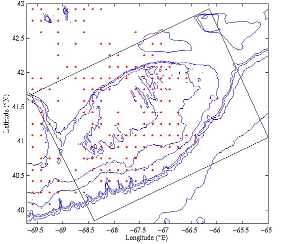
The operational system will consist of three nested domains: the Northwest Atlantic (NWA), the Gulf of Maine (GOM) and Georges Bank (GB). The specifics of the individual domains are given in Table VI-7 and the domains are shown in the figure below. In the operational context, there will be two-way nesting between the NWA and GOM (NWA/GOM) domains and the GOM and GB (GOM/GB) domains. The NWA/GOM nested run will provide boundary conditions for the GOM during the GOM/GB nested run.

Multiple model forecasts are required to produce each issued forecast. The update of the forecast is done in two stages. First a hindcast is done to bring the atmospheric forcing and assimilation up to date. Then a 12-day simulation is performed to produce the desired 10-day forecast fields. The separation of the hindcast and forecast simulations maximizes the use of the most recent atmospheric forcing data/forecasts. The nested pair runs are staggered, with the NWA/GOM hindcasts/forecasts being done on the work day previous to the GOM/GB runs. This plan is based on the following assumptions:

• Limiting time factor is an estimated run time of 1hr 55min per model day in the enlarged GB domain. This yields an estimate of 23 hours required for the 12-day forecast run.
• 16 vertical levels provide sufficient resolution for biology.

-- This needs to be checked ASAP.

• Assimilation, nesting and the use of atmospheric forcing are all assumed to have a negligible affect on the run time.

-- This needs to be checked, especially the negligibility of adding nesting.

• Runs are launched upon the receipt of 000Z FNMOC fields, instead of waiting for 1200Z fields. This allows runs to begin in the morning and finish the following morning.

• All assimilation fields are prepared by the night before a hindcast/forecast run is begun.

Graphically, the forecast plan is illustrated by the following time-line:

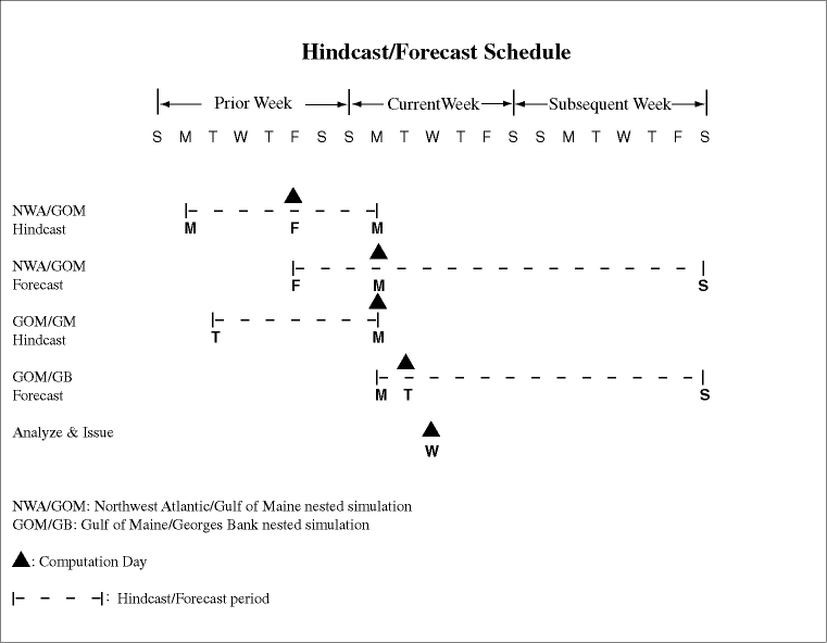
The GOM/GB forecast is actually a pair of runs. The first is a coupled physical/biological/fish dynamical model with complete data saved daily. The second is a physical model with sparse velocity data saved on quarter tidal cycles to save space.

SSH

-- Start from a relevant, previously created hindcast.

-- Adjust velocities from frozen TS fields (might not be necessary).

-- Adjust NPZ from frozen physical fields.

These adjustments will have to be done as soon as the SSC data are available. Because of the delay in getting SSC (~2 weeks), this will require additional hindcasts to bring fields up to date. Ramping will be done to get the data in within 1 day of the actual time.

The SST and SSC assimilation ramping time scales may have to be accelerated. It might prove necessary to assimilate the data only during the proper portion of the tidal cycle.

Atmospheric Forcing

° FNMOC fields will be collected at least twice daily.

-- CMAST is already doing this.

° Meteorological buoy data will be collected at least daily.

-- CMAST is developing an automated capability for doing this.

Satellite

° SST will be collected at least daily.

-- CMAST is already doing this.

° SSC will be collected at least daily.

-- CMAST is already doing this.

° SSH will be downloaded from Colorado at least daily.

° Fronts and Eddies analyses will be performed daily

-- CMAST has the collection capability.

in situ

° If any in situ data becomes available, it should be collected immediately.

Quality Control

• SST

-- CMAST has this capability for its image products.

• Corrections for skin effects need to be applied to bring SST in line with mixed layer

-- Under development.

• SSC

° Bad data values (land, clouds) need to be identified and flagged.

• SSH

° Regions of reliable SSH need to be determined and the data from those regions selected.

• Fronts

• The ordering of the discrete frontal locations needs to be checked and corrected,

° The local curvature in the frontal locations is smoothed by filtering.

-- Harvard has the necessary software

• FNMOC

° Comparisons with meteorological buoy data need to be checked.

Preparation

• FNMOC

° Need to be extended with climatological fields.

• Combine to form wind stress, net heat flux, evaporation minus precipitation and

• SST

• Smooth SST fields and sub-sample so data set will contain ~200 profiles (small enough to be objectively analyzed).

° Extend as constant profiles to the base of the mixed layer.

. FNMOC fields

. Previous model runs

• SSC

° Smooth SSC fields and sub-sample so data set will contain ~200 profiles (small enough to

be objectively analyzed).

° Construct first guesses for remainder of biological fields from statistical correlations.

° Adjust biological fields from frozen physical fields.

• SSH

Use Lozano's EOF procedure to adjust Gulf Stream FM fields in accordance with SSH.

• Grid shelf and slope/deep waters separately
• Shelf fields from data (SST, SSC, in situ) and Gulf of Maine FM

• Slope/Deep fields from Gulf Stream FM and SSH
• Meld with Shelf/Slope FM

1. Events

• January 1 - Models are closed

• February 1 - OSSEs are completed

• February 15 - Pre-operational forecasting begins

• February 29 - First SSC data of pre-operational period is available

• March 15 - Real-time operational forecasting begins

1. Resource allocation

• Hindcasts/forecasts for issuance are performed on CMAST computers in order to ensure rapid turn-around time

• Data preparation, sensitivity studies, etc. are divided amongst available Harvard and CMAST computers

1. Communication

• All data and model fields are shared across the Internet

5. Observation System Simulation Experiments (OSSE): Design and Execution

This section describes OSSEs to be conducted in order to improve overall system performance; to calibrate multidisciplinary models and operational protocols; to understand sensitivities; and to identify significant and critical parameters and procedures as related to the overall quality, accuracy and timeliness of real-time operations for the Spring 2000 AFMIS demonstration of concept.

The observation system is first defined in terms of the specific datasets, models and procedures to be used in the OSSE. This activity will be performed on the operational system components after their development test and initial tuning for this system. Other research activities that might impact into the scope and performance of the operational system are not considered in this document. An initial description of the operational system is given below. Each experiment will focus on addressing or testing 2-3 technical issues and assessing model performance and quality of output. The major elements of the ocean prediction and simulation system assemble for the demonstrations of concept, together with some major requirements are as follows:

1. Data quality control/preparation and analysis of gridded fields for models. Requires data processing, preparation of physical, biological, fish, atmospheric fields for initialization, assimilation and forcing;
2. Short term (3 day) and long term (10 day) data driven forecasts of physical, biological and fish fields. Requires initial tuned models and data assimilation protocols for the Georges Bank (GB), Gulf of Maine (GOM), and the Northwest Atlantic regions (NWA); real-time protocols for the forecasting center (including model quality control, metrics of forecast quality; tuning and validation of fish model(s) and near real-time protocols to prepare fish fields for initialization; possible data updates (assimilation), and forecasts. The various dynamical models will be at different levels of validity.
3. Products: distribution, model visualization, discussion and interpretation. Requires preparation of products for distribution and products for internal use during operations.
4. Near real-time acquisition (if possible) of real-time data, including physical, lower trophic levels and fish. Requires ship time, able-bodied sea personnel, resources for data transmission, operational protocols.

The OSSE design includes: A) Identification of operational system components (what is being tested); B) Description of real-time operations (how it supposed to work); C) Description of the experiments to be carried out (what tests are needed); and D) Execution: work tasks and schedule (how and when).

1. Operational system components - Data sets, procedures and models for the operational system are not completely defined, or are either under development, test, tuning and calibration. These will not be defined here.
2. Description of real-time operations - these activities can be gleaned from the section on Operational Protocols

C) Experiments

i) Near real-time acquisition

The activities under this heading will not be tested during the OSSE.

Data sets for initialization, assimilation, forcing and verification will be for the period of March 15 - April 15 1998.

ii) Data quality control / preparation and analysis of gridded fields.

Data preparation for models.

Experiment II.1 - Calibration of gridding parameters. Physics-Biology

Experiment II.2 - Construct initialization for physics and biology for 3 different configurations, using AVHRR combined with SeaWiFS to identify frontal positions. Adding complexity in each configuration. Integrations in model space to equilibrate biology.

Experiment II.3 - Calibration of gridding parameters. Fish. The final fields should be either close to equilibrium (near Z and comfortable T environment) or far from equilibrium with respect to one of the attractors. Integrations in model space to equilibrate fish distributions.

iii) Data driven forecasts

OSSE should be carried out only after initial tuning of the models and procedures involved. The term calibration should be understood below both, calibration and understanding sensitivity to a relevant set of parameters.

Experiment III.1 - Calibration of physical parameters and numerical parameters. The aim of this experiment is to obtain adequate representation of the following processes:

Large-scale circulation (including tidal residual circulation); (nesting, boundary and Shapiro parameters, tidal parameters)

Vertical mixing (including tidal mixing and wind mixing); (vertical viscosity and diffusivity parameters)

Frontal positions (dependencies on feature model derived fields, vertical mixing parameters)

Tidal advection (diurnal); (tidal parameters)

Experiment III.2 - Calibration of biological parameters and numerical parameters. The aim of this experiment is to obtain adequate representation of the following processes:

Large-scale PZ distribution (dependencies on initial and assimilation fields, u, nesting, boundary and Shapiro parameters)

Distributions of vertical structures of PZ (dependencies on biological parameters, w, mixing parameters)

P/Z ratios and productivity indices (dependencies on biological parameters)

Experiment III.3 - Calibration of fish parameters and numerical parameters.

Bank-scale fish distribution (dependencies on initial and assimilation fields, u, nesting, boundary (export-import) and Shapiro parameters)

Distributions of vertical structures of fish (dependencies on fish parameters, w, mixing parameters, vertical PZ distributions, T distribution)

Swimming behavior as parameterized by up/down-gradient diffusion in temperature and zooplankton concentrations

iv) Products

Experiment IV.1 - During OSSE; generate prototype products in a real-time mode to secure timely flow of the information, and if appropriate feedback from potential end-users.

We plan to commence the OSSE's the first week of October 1999 and anticipate having tested the complete system by the last week in January 2000. Software is expected to be finalized by 1 January. Recall that models/procedures are required to have being initially tuned for the area before OSSE experiments commence.

In order to test each of the above system components, a progression of experiments will be conducted. Since the biological and fish modeling are likely to yield the greatest number of challenges, it is sensible to secure enough time and resources to address issues related to these components of the system during the OSSE period.

While any fastidious schedule is bound to require modification, the following provides a schedule for how the OSSE's may progress:

- Data preparation and quality control

#) Assemble suitable historical and climatological data sets for physics, biology, and fish in GB, GOM, NWA. OSSE period: spring of 1998.

- Calibration of gridding parameters for physics and biology

#) OA and forcing parameters for GB

#) PE feature model analysis and assimilation for each domain and their nested configurations.

- Calibrate assimilation parameters for satellite data

#) "value added" assimilation schemes for satellite data

- Calibration of physical forecast parameters

#) PE parameters for GB

#) physical feature model parameters for GB, GOM

- Calibration of gridding parameters for fish

#) OA and forcing parameters for GB

- Calibration of biological forecast parameters for GB

#) forecast parameters for GB

- Calibration of gridding parameters for physics and biology

#) OA and forcing parameters for standalone GOM, NWA

- Calibration of fish forecast parameters for GB

#) forecast parameters for GB

- Calibration of physical forecast parameters for standalone GOM, NWA

#) physical PE parameters for standalone GOM and NWA

- Calibration of biological forecast parameters for standalone GOM, NWA

#) biological PE parameters for standalone GOM and NWA

- Calibration of physical forecast parameters for two-way nesting between GB-GOM, and GOM-NWA

#) forecast physical and numerical parameters data

- Test model output visualization, interpretation and distribution systems

#) real-time presentation and distribution of model products

- Complete system evaluation

#) Evaluate and validate assimilation and forecast systems for physics, biology, and

fish for nested GB, GOM, NWA domains

#) Evaluate and validate quality control and distribution systems

Resources needed to support the AFMIS demonstration include data, models, hardware and personnel.

VI.1 Data

The required data are summarized in tables VI-1 to VI-5.

TABLE VI-1: REMOTELY SENSED DATA

TABLE VI-2: BIOLOGICAL DATA

TABLE VI-3: PHYSICAL DATA

TABLE VI-4: METEOROLOGICAL DATA

TABLE VI-5: FISHERIES DATA

VI.2 Computational Models

The computational models and interfaces are described in table VI-6. The domains in which these are implemented are described in table VI-7.

TABLE VI-6: COMPUTATIONAL MODELS

TABLE VI-7: DOMAINS

VI.3 Hardware

The hardware required to operate the system is specified in table VI-8.

TABLE VI-8: HARDWARE

VI.4 PERSONNEL

The personnel who will participate in the demonstration exercise are identified in table VI-9.

TABLE VI-9 PERSONNEL

AFMIS - Advanced Fisheries Management Information System

AVHRR - Advanced High Resolution Radiometer (measures ocean temperature)

CMAST - Center for Marine Science and Technology

CPUE - Catch Per Unit Effort

DOC - Demonstration of Concept

EOF - Empirical Orthogonal Function

FM - Feature Model

FNMOC - Fleet Numerical Meteorology and oceanography Center

GB - Georges Bank

GOM - Gulf of Maine

HOPS - Harvard Ocean Prediction System

N-P-Z - Nutrients-Phytoplankton-Zooplankton

NASA - National Aeronautic and Space Administration

NOAA - National Oceanic and Atmospheric Administration

NWA - Northwest Atlantic

OA - Objective Analysis

ONR - Office of Naval Research

OSSE - Observation System Simulation Experiment

SeaWiFS - Sea-viewing Wide Field of View Sensor (measures ocean color)

SSC - Sea Surface Color

SSH - Sea Surface Height

SST - Sea Surface Temperature

URI/GSO - University of Rhode Island/Graduate School of Oceanography

Research hypotheses:

1. There are important interactive processes between the physics, biology and fish dynamics and feedbacks.
2. The variations in fish abundance over 1-2 week time scales are important for fisheries management and fishing.
3. A fisheries dedicated ocean prediction system can nowcast and forecast the state variables of interest.

Research issues:

1. Relative importance of buoyancy, wind, tidal, and boundary forcings
2. The response and variabilities in circulations that advect, mix and exchange.

1. relationship of synoptic scale to seasonal scale
2. topographic effects on dynamics
3. surface exchange on pelagic fish dynamics

1. Taking into account the physical processes, it is the relative influence of advection, mixing and water mass dynamics on biology and fish dynamics.
2. Limiting factors for primary production efficient representation of the ecosystem and population dynamics by the state variables via aggregated state variables.

1. chlorophyll dynamics
2. color dynamics

Concepts:

• relative effects of buoyancy verses wind forcing
• effect of wind forcing on surface circulation and effect on biology
• horizontal transport of biological material, horizontal tidal mixing, circulation, advection, storms
• relationship of synoptic/mesoscale to seasonal circulation
• dynamical description qualitative + quantitative of the O(days/2 +) variables
• bottom boundary layer physics verses benthic fish dynamics

• what are optimal numbers of boxes in ecosystem model to represent biology?
• advection of nutrients from North side of Georges Bank verses tidal mixing
• identify minimal, optimal, and maximal models
• interpretation and use of chlorophyll dynamics from SeaWiFS
• interpretation and use of color dynamics
• open verses closed ecosystem dynamics
• limiting factors for PZ

• determine variability in fish distribution (evaluate) over forecast time frame
• transport via ring and other slope feature events and internal effects on recruitment.
• development of benthic and pelagic fish models
• interactions among species
• optimal fish state variables
• modeling effects of fishing dynamics and processes (fishing & fishing management)

Processes of importance: